Zero-Knowledge: Turning Computation into Polynomials (Part 1/3)
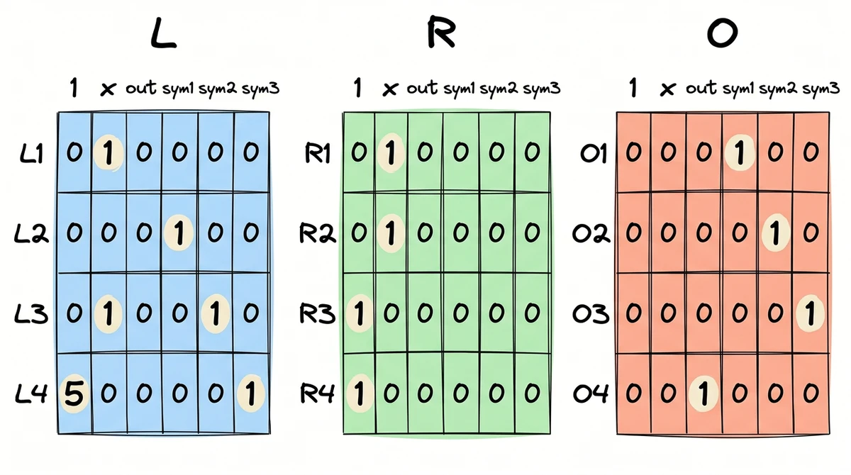
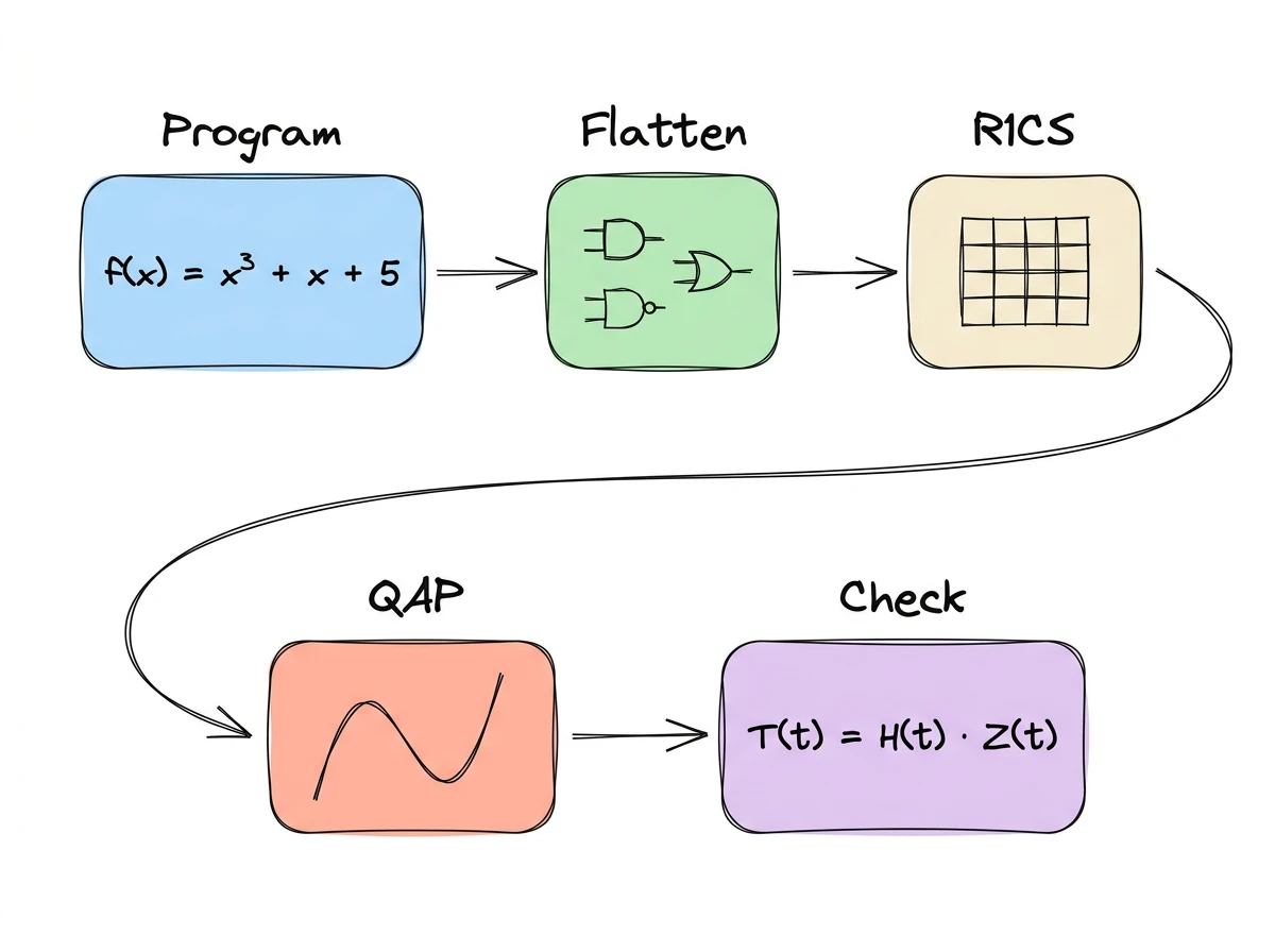
From a program to a few polynomial equations: how SNARKs encode computation through flattening, R1CS, and the QAP transformation Zero knowledge keeps coming up. Balaji frames it as the counterweight to AI: "Artificial intelligence is the attack. Zero knowledge is the defense." Podcasts, conference talks, crypto roadmaps: ZK is everywhere. I wanted to understand what's actually going on under the hood, so as promised, I traced the math from scratch. The part that excited me most wasn't the cryptography. It was the step before: how do you take a program and turn it into something cryptography can even work with? That's what this post covers. We'll take a small program, break it into elementary operations, encode those operations as matrices, and collapse everything into a single equation that a SNARK1 can check. The structure and example follow Vitalik's 2016 QAP walkthrough, which remains one of the clearest primers on the topic I could find. This is Part 1 of three (Part 2 covers the proof protocol, Part 3 covers applications). I'll assume familiarity with finite fields and polynomial commitments from my earlier posts. Alice claims she knows some value $x$ such that $f(x) = y$. Bob wants to be convinced, but he doesn't want to run $f$ himself (maybe it's expensive), and Alice doesn't want to reveal $x$ (maybe it's secret). A zero-knowledge proof gives them both what they want: Our running example for the entire post: $$f(x) = x^3 + x + 5$$ Alice claims she knows an input that produces 35. By the end of the post, we'll have transformed this claim into a single polynomial divisibility check. We'll use the actual solution $x = 3$ as we work through each step, but remember: in a real proof, this value is hidden from Bob. Step one is to break the computation into pieces small enough to encode as constraints. The idea is to rewrite $f(x) = 35$ as a sequence of elementary operations, each of the form Each line is a gate. The full set is an arithmetic circuit. The process of encoding computation as gates is called arithmetization, and it's the first stage of the SNARK pipeline. The flattened form encodes exactly the same logic as $f(x)$. Just a different representation. Our example is a cubic equation, but this flattening technique generalizes to any bounded program. Addition and multiplication over a finite field are expressive enough to encode conditionals, comparisons, and bitwise operations. For example, given a variable $b$ that's 0 or 1, the expression $y = 7b + 9(1 - b)$ picks one of two values: an Back to our example. We have four gates, and the next step is to express each one as a constraint that a verifier can check. Each gate becomes a constraint on a single shared vector. The format is called a Rank-1 Constraint System (R1CS). All the arithmetic from here on happens over a finite field $\mathbb{F}_p$. We use small integers to keep the example readable, but in practice $p \sim 2^{255}$. The vector $\mathbf{s}$ is a flat list of every variable in the circuit: $$\mathbf{s} = [1,\ x,\ \text{out},\ \text{sym1},\ \text{sym2},\ \text{sym3}] \tag{1}$$ With $x = 3$: $$\mathbf{s} = [1,\ 3,\ 35,\ 9,\ 27,\ 30]$$ That leading $1$ isn't a variable: it's a constant term that we'll see in action when $\text{gate } 4$ encodes the "+ 5" from the cubic equation. This vector, with all its intermediate values filled in, is the witness: it's everything the prover computed. Each gate becomes a constraint of the form: $$(\mathbf{L}_i \cdot \mathbf{s}) \times (\mathbf{R}_i \cdot \mathbf{s}) = \mathbf{O}_i \cdot \mathbf{s} \tag{2}$$ where $\mathbf{L}_i$ (left input), $\mathbf{R}_i$ (right input), and $\mathbf{O}_i$ (output) are the $i$-th rows of matrices $L$, $R$, and $O$. Each row vector "selects" the right variables from $\mathbf{s}$. $\text{gate } 1$ is $\text{sym1} = x \times x$. Looking back at $\mathbf{s}$ from equation $(1)$, we need vectors that select $x$ on the left, $x$ on the right, and $\text{sym1}$ as the result: $$\mathbf{L}_1 = [0, 1, 0, 0, 0, 0] \quad \text{(selects } x \text{)}$$ $$\mathbf{R}_1 = [0, 1, 0, 0, 0, 0] \quad \text{(selects } x \text{)}$$ $$\mathbf{O}_1 = [0, 0, 0, 1, 0, 0] \quad \text{(selects sym1)}$$ Check: $(\mathbf{L}_1 \cdot \mathbf{s}) \times (\mathbf{R}_1 \cdot \mathbf{s}) = 3 \times 3 = 9 = (\mathbf{O}_1 \cdot \mathbf{s})$. It works. $\text{gate } 2$ ($\text{sym2} = \text{sym1} \times x$) follows the same multiplication pattern: $\mathbf{L}_2$ selects $\text{sym1}$, $\mathbf{R}_2$ selects $x$, and $\mathbf{O}_2$ selects $\text{sym2}$. $\text{gate } 3$ has no multiplication: $\text{sym3} = \text{sym2} + x$. We encode it as $(\text{sym2} + x) \times 1 = \text{sym3}$, folding the addition into the $\mathbf{L}$ vector. The right side is just the constant $1$: $$\mathbf{L}_3 = [0, 1, 0, 0, 1, 0]$$ $$\mathbf{R}_3 = [1, 0, 0, 0, 0, 0]$$ $$\mathbf{O}_3 = [0, 0, 0, 0, 0, 1]$$ Check: $(27 + 3) \times 1 = 30$. $\text{gate } 4$ ($\text{out} = \text{sym3} + 5$) works the same way, with $\mathbf{L}_4 = [5, 0, 0, 0, 0, 1]$. Check: $(5 + 30) \times 1 = 35$. The key insight: additions don't add constraints. They ride along in the $\mathbf{L}_i$ or $\mathbf{O}_i$ vectors of existing gates. If the original computation had been $(\text{sym2} + x) \times 2$ instead of a pure addition, that would still be one gate: $\mathbf{L}_i$ selects $\text{sym2} + x$, $\mathbf{R}_i$ selects the constant $2$, and the addition costs nothing extra. The constraint count is driven by multiplications; additions just come along for free. Each row is a gate, each column an entry in $\mathbf{s}$. A valid witness satisfies all four instances of equation $(2)$ simultaneously. An invalid witness (e.g., wrong intermediate values, wrong output) fails at least one. We've now established that R1CS works, but also that it requires checking each gate separately: four checks for four gates, each requiring three dot products and a multiply. The Quadratic Arithmetic Program (QAP) transformation converts those four separate R1CS checks into a single polynomial divisibility check. The technique: take each column of the L, R, O matrices and turn it into a polynomial via Lagrange interpolation. The Verkle trees post already covered this: encoding discrete values as evaluations of a polynomial. Same trick, different data. Concretely, column $j$ of matrix $L$ has 4 values (one per gate). Treat these as evaluations at points $t = 1, 2, 3, 4$ and interpolate a degree-3 polynomial $L_j(t)$.2 For example, the $x$-column of $L$ has values $[1, 0, 1, 0]$, so $L_1(t)$ is the unique degree-3 polynomial passing through the points $(1, 1),\ (2, 0),\ (3, 1),\ (4, 0)$. Repeat for every column of L, R, and O. Result: 6 polynomials each for L, R, and O (since $\mathbf{s}$ has 6 entries; 18 polynomials total). We want a single polynomial that, at each gate point $t = i$, evaluates to the dot product $\mathbf{L}_i \cdot \mathbf{s}$. A useful property makes this possible: a weighted sum of polynomials is itself a polynomial. The weights just scale and combine the coefficients. So we can use the witness entries $s_j$ as weights on the column polynomials: $$L(t) = \sum_{j=0}^{5} s_j \cdot L_j(t)$$ $$R(t) = \sum_{j=0}^{5} s_j \cdot R_j(t)$$ $$O(t) = \sum_{j=0}^{5} s_j \cdot O_j(t)$$ At any gate point $t = i$, $L(i)$ evaluates to $\mathbf{L}_i \cdot \mathbf{s}$, the left-hand dot product for gate $i$. The same holds for $R(i)$ and $O(i)$. One polynomial per side (3 total), encoding all four gates at once. For a valid witness, every gate constraint holds, so $L(t) \cdot R(t) - O(t) = 0$ at $t = 1, 2, 3, 4$. Call this expression $T(t)$. It's a polynomial with roots at $1, 2, 3, 4$. Define the target polynomial $Z(t) = (t-1)(t-2)(t-3)(t-4)$, which has roots at those same four points. Since $T(t)$ and $Z(t)$ share the same roots, $Z(t)$ divides $T(t)$ with no remainder. The prover can perform polynomial long division to obtain a quotient polynomial $H(t)$ such that: $$T(t) = H(t) \cdot Z(t) \tag{3}$$ If even one gate constraint were violated, $T(t)$ would lose a root, the division would leave a remainder, and no polynomial $H(t)$ would exist. The Schwartz-Zippel lemma makes equation $(3)$ powerful: evaluate equality of both sides at a random $\tau$ to verify a computation; if the polynomials differ, the chance of accidentally passing is negligible.3 One random evaluation replaces all $n$ gate checks. Production circuits have millions of gates (Zcash Sapling uses ~1.5 million, zkEVM rollups tens of millions). That's where the "succinct" in SNARK comes from. The naive approach would be to send $T(t)$ and $H(t)$ to the verifier and let them pick $\tau$. But these polynomials have degree proportional to the number of gates: $O(n)$ data on the wire, and $O(n)$ work for each verifier to evaluate them. We just collapsed $n$ gate checks into one evaluation; shipping the polynomials would undo those savings. So we want the prover to evaluate and send only point results. Two problems stand between the QAP and an actual proof. The prover must not know $\tau$. If they do, they can compute $Z(\tau)$ (which is public), pick any $H(\tau)$, set $T(\tau) = H(\tau) \cdot Z(\tau)$, and satisfy equation $(3)$ without a valid witness. The prover must evaluate at $\tau$ without learning what $\tau$ is. The prover must be bound to the circuit's polynomials. Even with a hidden $\tau$, nothing forces the prover to evaluate the QAP's actual polynomials. They could fabricate unrelated ones that pass the check at the hidden point. Part 2 will add the cryptography that resolves both problems: a trusted setup that hides $\tau$, pairing-based checks that bind the prover to the circuit's polynomials, and a blinding step that makes the proof reveal nothing about the witness. Succinct Non-interactive ARgument of Knowledge. ↩ We use $t$ for the polynomial variable to avoid collision with $x$, which is already the circuit input. ↩ If $P$ and $Q$ are distinct polynomials of degree at most $d$ over $\mathbb{F}_p$, their difference $D = P - Q$ is non-zero with degree at most $d$, so it has at most $d$ roots. A random evaluation point lands on one of those roots with probability at most $d/p$. With $p \sim 2^{255}$ and $d$ in the thousands, this is negligible. ↩
Proving Without Showing
Flattening: Breaking Computation into Gates
result = left (op) right. Think of it as disassembling a formula into its simplest possible operations:sym1 = x * x // gate 1: squaring
sym2 = sym1 * x // gate 2: cubing
sym3 = sym2 + x // gate 3: addition
out = sym3 + 5 // gate 4: add constant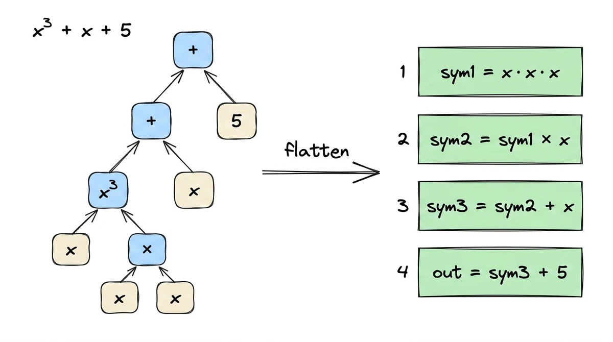
if/else built from arithmetic. Loops unroll to a fixed depth. The gate count grows with program complexity, but the encoding stays the same.R1CS: Constraints as Dot Products
Gates 1 and 2: encoding multiplication
Gates 3 and 4: encoding addition
The Full Matrices
QAP: From Dot Products to Polynomials
What One Equation Buys Us
What's Missing
This post was written in collaboration with Claude.